
On the Minimization of Expected Checkout Time
Covid-19 has had devastating effects, across cities, counties, states, and countries. But, in addition to its most life changing and paradigm shattering consequences, we’ve also seen subtler changes: vivid dreams are the new norm, more people are adopting puppies, and video games are now good for us. It may seem insensitive to think about these side-effects, given their triviality in the face of loss of life orders of magnitude greater than that of 9/11. How can we talk about puppies when two football stadium-fulls of Americans have succumbed to the deadliest and least understood virus since the Spanish Flu?
I join all 7.7 billion of my fellow world citizens in surprise, confusion, fear, sadness, and occasionally anger. But sometimes it’s nice to allow our minds a break from the cyclic coverage of portable morgues, business graveyards, and staggering numbers; so consistently high that they no longer seem staggering.
Today, I want to talk about the MOST DEVASTATING effect yet of COVID: I can no longer see the ends of checkout lines at my local Fred Meyer supermarket. The six to ten foot gap between register and shopping aisle is room-for-one only. Instead of picking lines based on their length, I’ve had to resort to randomly picking an aisle! I know. Absolutely devastating.
BUT, as they often do, these constraints offer an opportunity to take a more creative approach. Maybe some creativity combined with mathematical reasoning will allow for an opportunity of optimization that lets us beat, in expectation, our pre-pandemic wait time. How’s that for seeing the silver lining?
The Problem
You’ve just finished your grocery shopping, and walk down your aisle to see a horrifying sight: a long line of carts has built up in this aisle. You walk down to the front and turn to your right (you happen to have walked down the left-most aisle). The length of every line is hidden by a shopping aisle. You can stay in this aisle, or you can choose to walk down the corridor of registers. At each one, you can see only the length of that line. There’s not enough room to make a U-turn, so every time you walk past a register, you abandon it as an option. What strategy minimizes expected length of the line you end up in?
More formally:
\[\begin{aligned} N &:= \text{total number of carts} \\ L &:= \text{total number of lanes} \\\\ X_{L,N} &:= \text{The number of carts in our final choice lane given that }\\ &\quad \quad \text{there are $L$ lanes and $N$ carts left} \\ \end{aligned}\]We’re looking for a strategy which minimizes:
\[E[X_{L,N}]\]In words, this is the expected value of the length of the line we end up in, given no knowledge yet about how many carts are in any specific line.
Assumptions
This problem can have many degrees of complexity without some restrictions. We need to be able to make predictions about the probability distributions of future line lengths in order to calculate expected value. That means having information about $N$ and how those $N$ people are distributed among the checkout lanes. For my first go at the problem I’ve decided make several simplifying assumptions:
- Knowledge of $N$. This is pretty unrealistic, so I’m not going to try to defend it.
- In my second go, I plan on changing this assumption to “having some prior knowledge about $N$”, say a poisson prior (since number of people at a grocery store can be seen as a ‘rare event,’ in that there’s a lot of people who could be at the store, but each person at any given time has a very low probability)
- The people distribute themselves multinomially; i.e. each person has equal probability of ending up in any of the $L$ lanes. This is based off the assumption that a person has equal chance of ending their shopping in any of the lanes, and that most people will stay in the lane that they start in due to unavailability of the information needed to decide to switch lanes.
- The number of carts in the checkout lanes stays static throughout our search process.
- $L$ is known.
Also, to simplify the problem, I’m assuming that I don’t know anything about the length of the lanes which I haven’t checked (even though in reality I get a little bit of information when I see that there is/isn’t a cart between the register and the aisle).
The Math Part
An example is usually the best way to start
I’ve learned from experience—hours of attempting to solve problems with, and getting lost in, pure symbol shunting only to figure them out immediately after considering a trivial example—that the brain is much better at solving problems by extrapolating from simple examples than by thinking purely in generalizations. This proved true once again.
To start off with, consider the example where $N=6$ and $L=2$. That is, there are $6$ carts in total, distributed over $2$ lanes. However many carts are in the first lane fully determines the number in the second lane. This observation means that, once I see how many carts are in the first lane ($N_1$), the problem becomes deterministic: I will choose the lane with less carts, so the final length is equal to $\mathrm{min}(N_1, 6 - N_1)$. To find the expected value, we sum over all the possibilities of $N_1$:
\[\begin{equation} \begin{aligned} E[X_{2,6}] &= \sum_{k=0}^6 Pr[N_1=k]*\mathrm{min}(N_1, 6 - N_1) \\ &= \sum_{k=0}^6 b(N,\frac{1}{2},k)*\mathrm{min}(N_1, 6 - N_1) \\ &= \sum_{k=0}^6 2^{-6}{6 \choose k}*\mathrm{min}(N_1, 6 - N_1) \\ &\approx 2.41 \end{aligned} \label{eq:example1} \end{equation}\]This is already a pretty nice result. The resulting expected value is 0.59 or about 20% less than the expected value of 3 that we’d get with random choice.
Extrapolating from the example
The goal of starting with an example is to notice any patterns that can generalize. In our case, we want to get rid of the dependence on our choices of $L$ and $N$. $N$ is easy to generalize. We can just replace all of the instances of $6$ with $N$, since the process for coming up with our expression for $E[X_2|D_2=6]$ did not depend on our choice of $N$. We could have as just as easily picked $N=4$ or $N=100$ and the process for calculating $E[X]$ would have stayed the same. This gives us:
\[E[X_{2,N}] = \sum_{k=0}^N 2^{-N}{N \choose k}*\mathrm{min}(N_1, N - N_1)\]$L$ is harder to deal with. Two parts of the calculation depended on our choice of $L$: $Pr[N_1=k]$ and $N-N_1$, the second term in the $\mathrm{min}$ function.
The dependence of the $Pr[N_1=k]$ term on $L=2$ is purely in the choice of probability in the $b(N,\frac{1}{2},k)$ coefficient. In case of general $L$, the probability of any given person ending up in lane one is $\frac{1}{L}$ (due to our assumption of equal probability across all lanes). This gives us $Pr[N_1=k] = b(N, \frac{1}{L}, k)=(1/L)^k(1-1/L)^{N-k}{N\choose k}$.
The minimization term is harder to deal with. The second term of the minimization ($N-N_1$) depended on the fact that, given knowledge of $N_1$, we knew exactly how many carts would be in the last lane. With general $L$ we don’t have that luxury.
Once again, it helps to look at an example. Consider $N=8$ and $L=3$. If $N_1=2$, we end up in the exact situation as before, with $6$ carts and $2$ lanes left. In this case, we’re presented with the decision to stay and be guaranteed a wait time of $2$ carts, or continue and wait for $2.41$ carts in expectation. So our optimal choice would be to stay. If we had seen $3$ carts in lane $1$, our optimal choice would have depended instead on $\mathrm{min}(3, E[X_{2, 5}])$.
In general, if we know the expected value of the optimal strategy when $L=L-1$ and $N=N-N_1$, we can make the informed decision of choosing the minimum between $N_1$ and said expected value.
\[E[X_{L,N}]= \begin{cases} N & L=1 \quad\text{our base case, when 1 lane is left} \\ \sum_{k=0}^N b(N, \frac{1}{L}, k)\mathrm{min}(N_L, E[X_{L-1,N-k}]) & L > 1 \end{cases}\]We can check that plugging in $N=6$ and $L=2$ gives us exactly the expression as in $\eqref{eq:example1}$.
As Professor Venkatesh would say, at this point we have exhausted all the probability. Sadly, probability didn’t give us a nice, closed form expression to provide intuition as to what this crazy expected value expression actually looks like in practice. So instead, let’s whack it and see what fruit falls.
Finding optimal expected cart count
Our recursive expression for expected value makes it an ideal candidate for dynamic programming. It obeys the requirements that:
- Complete solutions can be calculated from optimal solutions to subproblems
- There’s a logical order to fill the DP table (in order of increasing $L$ and $N$)
The DP has size $L \times N$. Calculating each expected value term in the table takes $O(N^2)$ time since we’re summing $O(N)$ terms and the binomial coefficient in each term takes $O(N)$ time to calculate (assuming constant time multiplication). The overall $O(N^3L)$ time is perfectly feasible since I can’t imagine any cases where $N$ would be significantly higher than 100, or $L$ higher than 20 (which would require operations on the order of $2\times 10^7$).
The Code
Due to the convenient structure of $E[X_{L,N}]$, the translation into python is simple:
## binomial(total number, probability, number of successes)
def binomial(n: int, p: float, k: int):
    return math.comb(n, k) * math.pow(p, k) * math.pow(1 - p, n - k)

# creates a dp table for expected value when there are i lanes and j people left
def expected_carts_table(N: int, L: int):
    # dp table, L x N
    dp = [[math.inf for j in range(0, N + 1)] for i in range(0, L + 1)]

    # initialize base case
    # number of people in the last lane must be the number of people left
    dp[1] = [j for j in range(0, N + 1)]

    # loop from low L (N) to high L (N)
    for i in range(2, L + 1):
        for j in range(0, N + 1):
            p = 1 / i
            v = [binomial(j, p, k) * min(k, dp[i - 1][j - k]) for k in range(0, j + 1)]
            dp[i][j] = sum(v)

    return dp
Above: binomial calculates probability of k successes over n events, giving single success probability p. expected_carts_table generates the DP table as in [insert reference]
(Note: All code can be found in this repo. Jupyter notebook is at the bottom of the page)
The Results
I really hate that there isn’t a closed form (that I know of). Closed form often translates one to one to a nice English description of the behavior of the dependent variable ($E$) in response to the inputs ($N$ and $L$). As a plan B, visualization turned out to show some pretty patterns.
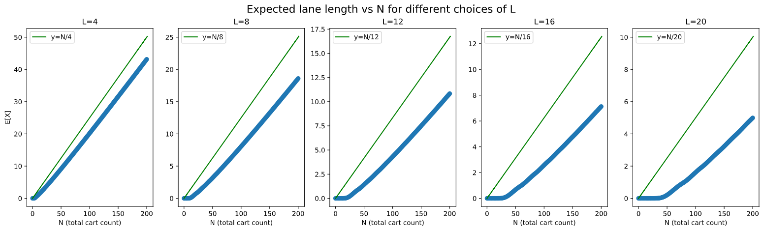 y-axis scales are not the same across the graphs. It’s decreasing with increasing $L$. The green line represents average cart count per lane.
The graphs above show a very clear linear relationship between increasing $N$ and $E$, though with a weird little foot of 0s at the start, almost like a hocky stick or a shifted ReLu (since for $N$ up to $L-1$, by the pigeonhole principle, there will always be an empty lane. And for $N$ not much larger than $L$, the probability of an empty lane remains high).
The line in each of the graphs represents what expected lane length looks like in the random choice strategy. The optimal strategy already does better in the case of $L=4$, and the gap increases as $L$ increases.
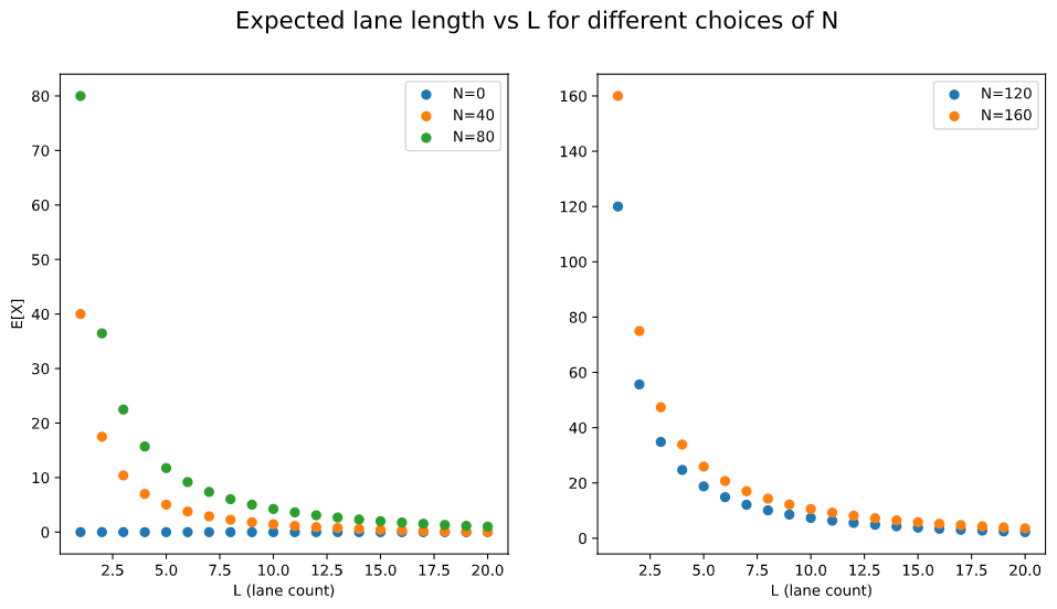
This graph looks at it from the other perspective. It shows, for different choices of total cart count, how the expected result varies with the number of lanes. As $L$ increases, there looks to be some sort of asymptotic decay, with its asymptote at $y=0$.
We can verify this with an application of the squeeze theorem. The function for $E[X]$ is obviously, and I don’t take using the word “obviously” lightly, lower bounded by 0. And since an optimal strategy must always perform at least as well as a random strategy—proof left as an exercise for the reader :)—it’s upper bounded by $\frac{N}{L}$. For example, with $N=120$:
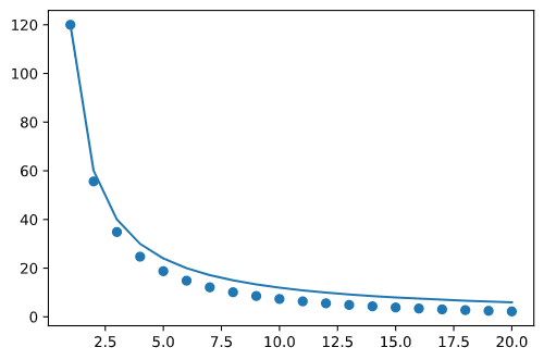
So because $\frac{N}{L}\rightarrow 0$ as $L\rightarrow\infty$, $E[X]$ must tend towards $0$ as well.
Perhaps a better way to directly compare the optimal strategy versus random chance is to fix one of them. To do this, I graphed the ratio between the expected values of the optimal strategy vs random choice with fixed $N/L$ (i.e. expectation given random choice).
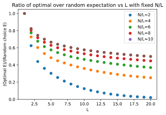
It’s clear that the more opportunities to choose we have (i.e. the more lanes there are), the better our strategy does in comparison to random choice. What’s less clear is if this advantage, quantified by the ratio of expectation in the optimal strategy vs random choice, always tends to zero. I’ve yet to give this question much thought, but at first glance it seems to be a very difficult problem; probably intractable given my limited undergraduate mathematical arsenal. If you know of a way to approach this, please let me know.
Number of lanes checked
Another logical question to ask here is: in expectation, how many lanes do I need to check?
The Math Part. Part 2
The math here plays out in a similar fashion to the first part. Define the following random variable:
\[W_{L,N} := \text{number of lanes checked (using optimal strategy) for $L$ and $N$}\]As before, we can partitian based on how many carts are in the first lane. For any given possibility, say $i$, for that number, we can tell whether our strategy was to keep going, or stay put, purely by checking the expected value table we got in the first section. If $i\leq E[X_{L-1,N-i}]$—i.e. the expected wait time is higher if we keep going than the guaranteed wait time if we stay—then we stayed put. Otherwise, we kept going. In the case that we stayed put, $W_{L,N}=1$. In the case that we kept going, $W_{L,N}=1 + W_{L-1,N-i}$. This can be codified in notation as follows:
\[\begin{aligned} f(L,N,i) &=\begin{cases} 1 & i\leq E[X_{L-1,N-i}] \\ 1 + W_{L-1,N-i} & i > E[X_{L-1,N-i}] \end{cases}\\ E[W_{L,N}] &= \begin{cases} 1 & L=1 \quad\text{our base case, when 1 lane is left} \\ \sum_{k=0}^N b(N, \frac{1}{L}, k) f(L, N, i) & L > 1 \end{cases} \end{aligned}\]The Code
And it can be codified, literally, as follows:
EPSILON = 10 ** -12
# creates a dp table for expected number of lanes checked given the carts table from before
def expected_lanes_table(carts_table: List[List[float]]):
    L = len(carts_table) - 1
    N = len(carts_table[0]) - 1
    lanes = [[math.inf for j in range(0, N + 1)] for i in range(0, L + 1)] # initialize array
    lanes[1] = [1 for i in range(0, N + 1)] # initialize base case: 1 if we're in the last lane

    # loop from low L (N) to high L (N)
    for i in range(2, L + 1):
        for j in range(0, N + 1):
            p = 1 / i
            # terms in the sum for E[W]
            v = [binomial(j, p, k) * (1 + (0 if k <= carts_table[i-1][j-k] + EPSILON else lanes[i - 1][j - k])) for k in range(0, j + 1)]
            lanes[i][j] = sum(v)

    return lanes
The Results
Again, the lack of closed form makes visualization essential. First, we’ll look at the expectation versus $N$ for certain fixed $L$:
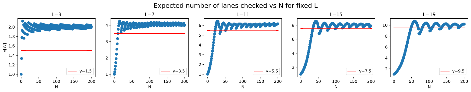
This is…not what I expected…. And I’m not really sure what to make of it. The expected value increases to a certain point (around $L/2$), then oscillates, discontuously, around it. The period of the oscillations is higher for larger $L$, and the amplitude decreases with increasing $N$. If anyone knows how to interpret this, please let me know.
Thankfully, visualizing the other direction (by fixing $N$ instead of $L$) results in an elegant, and interpretable, structure:
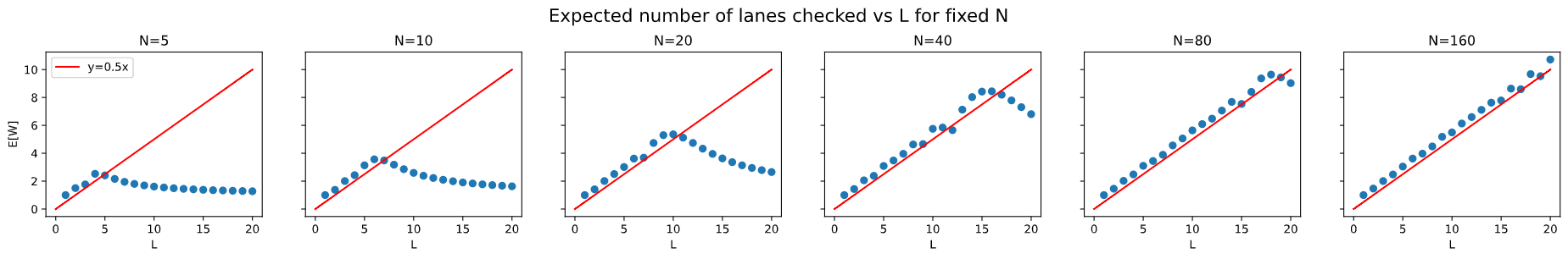
I noticed two main main things from this.
- For small $N$, we see a rise and then a fall. This is probably because as $L$ increases, it becomes more and more likely for the first lane to have 0 elements.
- Most striking is the linear relationship. The rising parts of the function, for any $N$, looks to have a slope around $L/2$. In other words, on average we have to check around half of the lanes. This provides a nice, elegant, and intuitive result to end things off.
Conclusions
I’ve always been drawn to math by its potential to discover (or invent, depending on your philosophy) beautiful underlying structures which aren’t apparent to the naked eye, or to the naked intuition. Drilling down on a seemingly innocent looking problem reveals surprising shapes, elegant results, and difficult next steps.
In a time when fact itself has become a partisan issue, I gain comfort in the solid axiomatic foundations and logical reasoning which math is…hold on, Gödel’s calling.
“Hey Gödel, what’s up?”
“Hmm. Mhmm, yeah that’s a clever way to number statements. What should I care though?”
“Okay, right, so I can perform variable substitution to get a new theorem and number. Got it.”
“Holy. You’re right. Then one could write, ‘this theorem is not provable’, IN THE SYSTEM ITSELF. Hilbert’s gonna absolutely flip”
Slowly puts down the phone. Casually looks around to make sure no-one’s watching…
Installs TikTok.