
When Games Become D̶u̶e̶l̶s̶ Duals
A game theoretic perspective on Lagrangian Duality
They say it’s unhealthy to see things as zero-sum… They are wrong (sometimes). In fact, zero-sum games can be incredibly useful. While it’s hard to say/prove things about games in general, even if restricting to two players, adding the constraint that players are strictly adversarial gives us enough structure to prove the minimax theorem—arguably the (second) most important theorem in game theory. Despite the extra structure, they’re still widely applicable. Zero-sum games are great for modeling excludable resources, and have been used as foundations for the theory of Generative Adversarial Nets (GANs) and online learning.
For me though, the most beautiful application (or perhaps recasting) of zero sum games, and most ubiquitous, is in optimization; where the minimax theorem pops up as a fundamental theorem relating optimization problems and their so called “duals”.
Games
Zero-sum games
A game is an interaction between two players. Each player chooses an action, and receives a reward or loss determined by the two actions. A zero-sum game is a game where for any given pair of actions, the amount one player receives is the exact negation of the other player.
For example, consider the matching pennies game. Each player picks a face (heads or tails). Alice’s goal is to play the same face as Bob, while Bob’s goal is to make sure they show different faces. In table format:
| A/B | Heads | Tails |
|---|---|---|
| Heads | +1, -1 | -1 , +1 |
| Tails | -1, +1 | +1 , -1 |
Note that writing down both players’ utilities was redundant. We can also represent the data by only writing down Alice’s loss (Bob’s utility).
| Heads | Tails | |
|---|---|---|
| Heads | -1 | 1 |
| Tails | 1 | -1 |
With this representation, we say the Alice is the minizer since she’s trying to minimize her loss, while Bob is the maximizer, since maximizing Alice’s loss is equivalent to maximizing his own utility.
Players don’t necessarily need to have a deterministic strategy, where they always pick heads, or always pick tails. A mixed strategy is a probability distribution over actions, so that utility now becomes expected utility. For example, an equilibrium mixed strategy profile in the matching pennies game has both players just flipping their coin (i.e. choosing heads/tails with probability 50%). Why is this an equilibrium? Say I’m Bob, and I know Alice is playing a uniformly random strategy. Then no matter how I play, there’s always going to be a 50% chance of matching. So I have no incentive to deviate. The same can be said about Alice.
The minimax theorem
The natural question when presented with any game, is: what is the ideal way to play? Is there even an ideal way to play? If there is, is it unique?
In the example of matching pennies, we saw that 50-50 was an equilibrium strategy. By playing head 50% of the time, Alice ensured that player could never do better than a utility of 0 in expectation. But could Alice have done better?
To make this question more concrete, let’s first consider the setting where there is an order of play. If Alice has to commit to a (mixed) strategy first, without knowledge of Bob’s strategy, how should she play? Clearly if she plays any pure strategy, Bob can take advantage of that and always play the opposite face. Even if she mixes, as long as there’s some bias, say she plays heads 51% of the time, Bob will be able to take advantage and win the majority of the time; in this case by playing tails. We therefore see that Alice’s best strategy, knowing that Bob will make a rational best-response, is uniquely to flip the coin.
One way to generalize this approach is that Alice’s goal is to make Bob indifferent between all his possible strategies. Since if Alice plays in such a way that Bob has an advantage playing Heads over Tails, due to the purely adversarial nature of the game, that means that Alice is not yet playing optimally.
There does seem to be something special going on in this example though, which a priori does not seem to be generalizable. If we instead flip the order and have Bob commit to a strategy first, and Alice best respond, the value of the game, the utility that Bob is able to guarantee himself in expectation, remains zero. In fancy math notation, this says, where $f$ represents Alice’s loss function:
\[\min_{a\in A}\max_{b\in B} f(a,b)=\max_{b\in B}\min_{a\in A}f(a,b)\]But clearly, in general, the player who goes second should have the advantage, right? They get to act with full knowledge of how their opponent is picking their strategy.
On the contrary, the minimax theorem says that the above formula is true for all zero-sum games. I.e. it is always equivalent to go in either order; there is a unique value to every zero-sum game. I won’t give a proof of this statement, but to get some intuition for it, I find it useful to look at it from the perspective of the graph of a game.
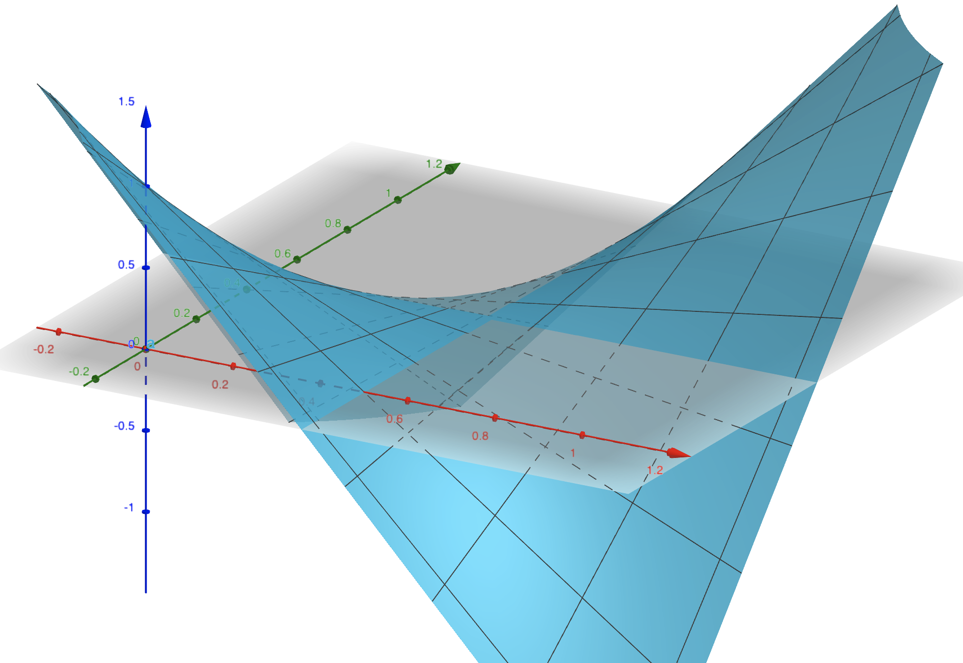
The above shows game Alice’s utility as a function of her probability of picking heads (the red axis) and Bob’s probability of picking heads (the green axis). The key feature of the graph is the saddle point at $(0.5, 0.5, 0)$. At this point, neither player has incentive to deviate. And it is the only point where this is true. Therefore, no matter if Alice or Bob goes first, they will choose the strategy corresponding to this saddle point. The claim is then that the graph of every finite zero-sum game has such a unique saddle point.
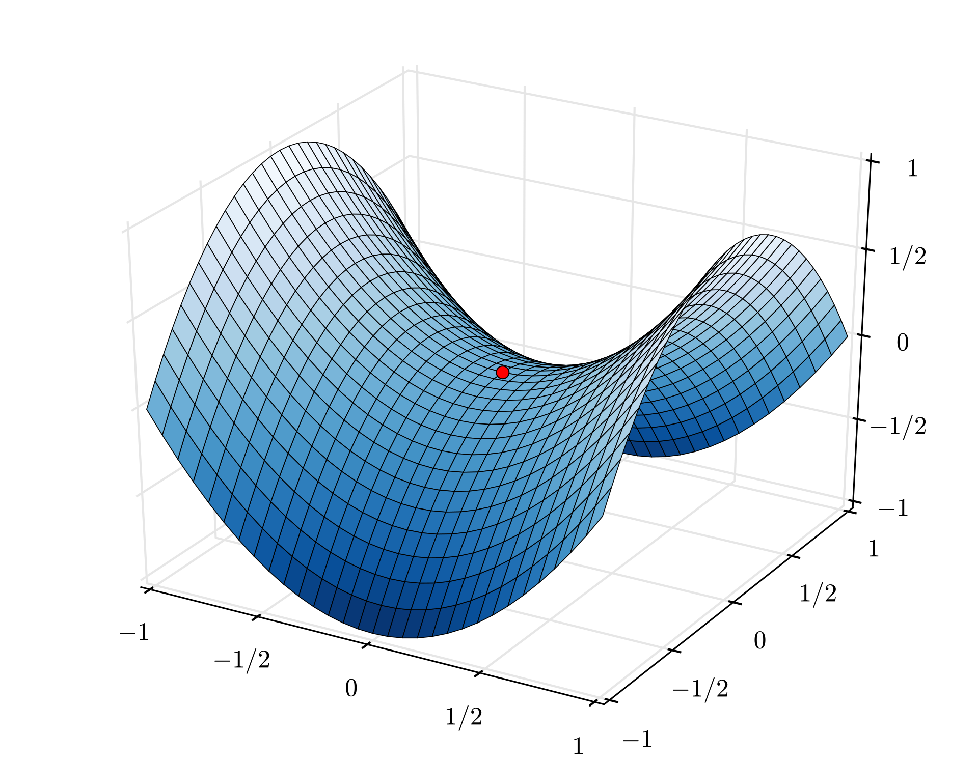
Actually, with this “graph of a function” perspective, we can intuit an even more general statement. One sufficient condition for the existence of saddle points (modulo attainment and boundary issues) is that $f$ is a convex-concave game lying over a convex strategy space. What this means is that, fixing $b$, $f(-,b)$ is convex in A’s strategy, and fixing $a$, $f(a,-)$ is concave in B’s strategy. Intuitively $f(-,b)$ looks like a U, while $f(a,-)$ is similar but flipped upside down. Via Wikipedia, such a graph looks like (with saddle point marked in red):
The case of finite games, such as matching pennies, can be seen seen as a specialization of this statement; where strategies live in the cross product of two $n$-simplices (a convex space), and the value of the game fixing one player’s strategy varies linearly (making it both convex and concave).
I hope this brief illustration provides some visual intuition for the minimax theorem. Another cool way of proving it (in the special case of finite games) is based on the existance of no-regret learning algorithms. See these lecture slides for such a proof.
Duals
Now let’s turn to a seemingly unrelated arena: convex optimization. Here, the goal is to minimize some loss function subject to constraints on the variables.
\[\begin{align*}\tag{1} \mathrm{minimize}_x\;& f_0(x) \\ \mathrm{subject\;to}\;& \forall_{i \in\{1,\dots,n\}}, f_i(x) \leq 0\\ & \forall_{j \in\{1,\dots,m\}} h_j(x) = 0 \end{align*}\]where $f_i$’s are all convex and $h_j$’s are all affine.
Examples abound: a data scientist or statistician minimizing least squares; a robotics engineering minimizing deviation from an ideal path subject to physical constraints (e.g. max turn frequency/size); an agent maximizing (i.e. minimizing the negative of) their utility under budget constraints.
Soft Constraints
The constraints above are in a sense as strict, or hard, as possible. One way to think of them is that if $x$ is chosen to violate a constraint, the cost immediately shoots up to positive infinity. An interesting question to ask is, what happens if, instead of enforcing this constraint “with infinite force,” you applied a more gradual, softer, cost; say, linear? So that the optimization problem becomes:
\(\begin{align*}\tag{2} \mathrm{minimize}_x\;& L(x,\lambda,\nu):= f_0(x) + \sum_i \lambda_i f_i(x) + \sum_j \nu_jh_j(x) \end{align*}\) where $\forall i,\; \lambda_i \geq 0$. Here, the $\lambda$ punishes any $f_i > 0$, while the $\nu$, being allowed to go in either the positive or negative direction, can punish any deviation from 0. Call the function above the “Lagrangian” of the optimization problem
Beyond being an intellectually interesting question, this is motivated by practical considerations as well. For instance, a regulatory institution (say, the EPA) may rather apply a cost to a company’s (say, Exxon) environment infractions rather than sending in the national guard to enforce them (which they probably can’t do anyways). Their goal then is to set the $\lambda$s and $\nu$s (the prices) in such a way that it’s in Exxon’s best interest to satisfy the constraints anyways. Which begs the questions: Do such prices exist? If they do, how do you find them?
Optimization is a game
The scenario with Exxon and the EPA above starts to make things sound like a “game” between two players with competing agendas. Is there a way we can bring this problem into the realm of zero-sum games? Well, I’m glad I asked, cause yes there is.
Take a look back at (1) and (2). I claim that (1) is equivalent to the following:
\[\min_x\max_{\lambda\succeq 0,\nu} f_0(x) + \sum_i \lambda_i f_i(x) + \sum_j \nu_jh_j(x)\]Why? Consider if Exxon violates some inequality constraint $f_i$. I.e. $f_i(x)>0$. Then the EPA can make Exxon’s cost unboundedly high by setting $\lambda_i$ unboundedly high. Similarly, if Exxon violates an equality constraint $h_j$, the EPA can set the $\nu$s unboundedly far in the direction of the infraction.
On the other hand, as long as Exxon satisfies all the constraints, the last term is $0$ no matter how the EPA sets $\nu$; while the highest the EPA can get the middle term is also to $0$, by setting $\lambda$ to uniformly zero (this motivates why we constrain $\lambda$ to be non-negative). Therefore, the problem then reduces to $\min f_0(x)$ (our original problem). Call this value, i.e. the solution to (1), $p^* := \min_x\max_{\lambda\succeq 0,\nu} L(x,\lambda,\nu)$.
Before applying minimax, we have to check that this function is convex-concave. Convexity w.r.t $x$ (player 1’s action) comes for free by assumption, while concavity comes for close to free by the fact that the expression is affine w.r.t $\lambda$ and $\nu$. And so…. the minimax theorem tells us that, IN FACT, the EPA can set their prices in such a way that the best Exxon can do is $p^*$, the value they achieve when satisfying the constraints. And what is this setting of their prices?
\[\begin{align*}\tag{3} \mathrm{maximize}_{\lambda,\nu}\;& \min_x(f_0(x) + \sum_i \lambda_i f_i(x) + \sum_j \nu_jh_j(x))\\ \mathrm{subject\;to}\;& \lambda_i \geq 0 \end{align*}\]This is exactly the famous Lagrangian dual problem from convex optimization. And the fact that the value of (3) is equal to $p^*$ (modulo feasibility) is exactly the fundamental strong duality theorem of convex optimization.
Another cool piece of intuition we can transfer from the game theory setting is the idea of “making your opponent indifferent.” In this case, the EPA is trying to set their prices in a way that the gradient of $L$ w.r.t $x$ is zero. I.e. Exxon is indifferent to changing its $x$ locally (and globally, is best off staying put because of convexity).
I think this connection is really sweet. When I first saw strong duality, I struggled to gain intuition for why we were doing what we were doing. Without the right framework from which to view it, the Lagrangian can look rather arbitrary. Looking at it from a game perspective provides a natural, intuitive framework.
We’ll conclude with a quick example.
A familiar example
Consider the following linear optimization problem:
\[\begin{align*} \mathrm{minimize}_x\;& 2x-1 \\ \mathrm{subject\;to}\;& 4x \geq 2 \end{align*}\]Yes, I know that $4x\geq 2$ is equivalent to $2x\geq 1$. I have my reasons, which will be revealed in time…
Next, we take the Lagrangian before dualizing.
\[L(x,y)=2x-1 + y(2-4x)\]Minimizing w.r.t $x$ after fixing $y$ (implicitly assuming a non-negative domain for $x$) gives the following dual problem:
\[\begin{align*} \mathrm{maximize}_y\;& 2y-1 \\ \mathrm{subject\;to}\;& 4y \leq 2 \end{align*}\]This is mildly interesting, as it seems like the primal and the dual problems are in a sense symmetric.
What’s more interesting is if we take a closer look at the Lagrangian: \(L(x,y)=-1+2x+2y-4xy = [x(1-y)-(1-x)y] - [xy + (1-x)(1-y)]\)
Interpret $x$ as probability that Alice picks heads, and $y$ as probability that Bob picks head and… Yes! It’s exactly the matching pennies game (this is why I chose to use $4x\geq 2$)! And we can easily check that the solution to the dual and primal give us $x=y=\frac{1}{2}$ with value $0$. Duals are games… and games are duals!
Conclusion
At the start of this post, I’d remarked that this is the most “ubiquitous” application of zero-sum games. I won’t go into too much depth (this is already a lot longer than I, and probably you too, hoped it’d be), but duality really has proved itself incredibly important. In convex optimization itself, the dual is used for sensitivity (how the optimal value changes with small perturbations of the constraints) analysis and to improve tractibility of a problem by transforming it from a problem with many variables and low dimension, to one with few variables.
It also pops up in graph theory, where the equivalence of flow maximization and cut minimization follows from the duality between the problems as linear programs. I think this example is especially cool; we get an important result in graph theory as an instantiation of another theorem which is fundamentally about competitive interactions between two adversaries. This is why I love math and computer science. The abundance of things which, at a first glance look completely unrelated, but beneath the surface are deeply entangled.
Life isn’t zero-sum, and even some games aren’t. But duels are, and though that might not’ve been good for Hamilton or Galois, it’s good for us.